What Format Do You Upload Data Sets to Rstudio in
Importing Datasets
A offset step in data assay is importing datasets. These can exist in several formats. Fortunately, R has several packages that allow us to easily import data from comma-separated value (CSV), SPSS and Excel files.
You volition find the following datasets on ILIAS:
- zufriedenheit.csv
- zufriedenheit-semicolon.csv
- zufriedenheit.sav
- zufriedenheit.xls
This is a generated dataset. The variables are a satisfaction rating, recorded at ii time points for four subjects.
zufriedenheit.csv is a text file, in which the columns are separated by commas (hence the name). zufriedenheit-semicolon.csv is likewise a text file, just with a semi-colon as the delimiter. zufriedenheit.sav and zufriedenheit.xls are SPSS and Excel files.
In your RStudio project folder in the file system of your estimator, create a new directory named 'information' and save the files you lot downloaded.
In RStudio, at that place are two ways of importing files:
-
Using functions:
read_csv(),read_csv2()(for ';' delimiters),read_sav()andread_excel(). -
Via the GUI: You can access this functionality either through 'File > Import Dataset' or in the Environs pane.
The 2d option is easier to use, and has the advantage that R will generate all code for importing datasets for us, which can be copied for subsequent use.
Comma-separated value (CSV) files
The functions nosotros need for importimg CSV files are available in the readr package. This needs to be loaded:
Alternatively, we tin can simply load all tidyverse packages:
library(tidyverse) We volition beginning import the information files using the GUI. In Surround, click on Import Dataset > From Text (readr) (or 'File > Import Dataset > From Text (readr)'). Y'all volition see a dialogue containing a Code Preview with the following lawmaking:
library(readr) dataset <- read_csv(Zilch) View(dataset) On the left (bottom) you lot will find all options for importing the data. These options are all arguments of the read_csv() function (or the more general read_delim() funtion):
args(read_csv) #> role (file, col_names = True, col_types = NULL, locale = default_locale(), #> na = c("", "NA"), quoted_na = TRUE, quote = "\"", annotate = "", #> trim_ws = TRUE, skip = 0, n_max = Inf, guess_max = min(1000, #> n_max), progress = show_progress()) #> Null In the File Browser you can select the zufriedenheit.csv file. Later doing so you will run across Information Preview.
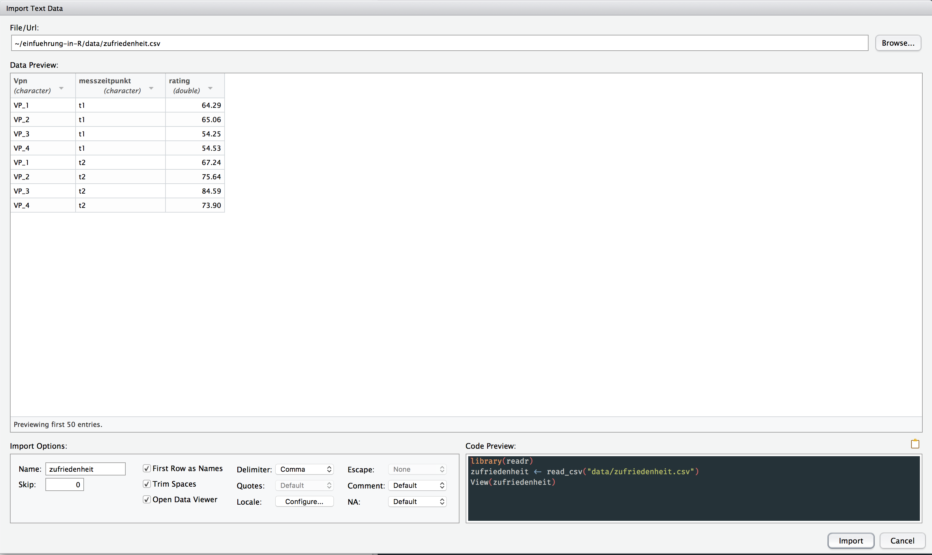
The variables Vpn and messzeitpunkt have been imported as character vectors. These volition demand to be converted to factors. Under Import Options a file name is generated automatically. This is simply the file proper name, minus the .csv suffix.
Endeavour to discover what happens when you play around with the options, east.g. "First Row every bit Names".
Now click on Import. A new data frame (tibble) with the proper noun zufriedenheit volition appear in the Surround pane, and the generated R code is printed to the console.
library(readr) zufriedenheit <- read_csv("data/zufriedenheit.csv") #> Parsed with column specification: #> cols( #> Vpn = col_character(), #> messzeitpunkt = col_character(), #> rating = col_double() #> ) We still have to convert the grouping variables to factors:
zufriedenheit$Vpn <- as.cistron(zufriedenheit$Vpn) zufriedenheit$messzeitpunkt <- every bit.cistron(zufriedenheit$messzeitpunkt) zufriedenheit #> # A tibble: 8 x three #> Vpn messzeitpunkt rating #> <fct> <fct> <dbl> #> 1 VP_1 t1 64.iii #> two VP_2 t1 65.1 #> 3 VP_3 t1 54.2 #> iv VP_4 t1 54.5 #> five VP_1 t2 67.2 #> 6 VP_2 t2 75.6 #> # ... with 2 more rows Now practice the same with the semi-colon delimited file zufriedenheit-semicolon.csv. This is something that yous frequently be confronted with if your calculator uses a High german locale.
You should see the following lawmaking in the Code Preview:
library(readr) zufriedenheit_semicolon <- read_delim("information/zufriedenheit-semicolon.csv", ";", escape_double = FALSE, trim_ws = True) Try importing both files using the R commnands. For the semi-colon file y'all can use the office read_csv2().
If you want to save a data frame as a CSV file, you tin can use the function write_csv():
write_csv(ten = zufriedenheit_long, path = "data/zufriedenheit.csv") SPSS datasets
Nosotros can import the same dataset, simply this fourth dimension from the SPSS file format (zufriedenheit.sav). There is a parcel called haven; this provides the office read_sav(). We can load the package to make the function available:
library(oasis) zufriedenheit_spss <- read_sav("data/zufriedenheit.sav") Just, equally before, we tin can as well use the GUI. In the Environs pane, click on Import Dataset > From SPSS, and choose the file. You volition see a Code Preview:
In contrast to importing CSV files, nosotros have no options when importing from SPSS except for the name of the data frame, which we volition change to zufriedenheit_spss.
Now yous can click on Import. In the Environs pane, the newly created varibale volition appear. Variables imported from SPSS tin can accept additional attributes, the most important of which is the labels aspect:
zufriedenheit_spss$Vpn #> #> [1] i 2 3 4 1 2 3 4 #> attr(,"format.spss") #> [ane] "F8.0" #> attr(,"labels") #> VP_1 VP_2 VP_3 VP_4 #> i 2 iii 4 This contains the SPSS value labels. Using this, we can look up what blazon of coding scheme was used for chiselled variables. If the values 0 and ane were used for the sex activity variable, nosotros determine which sexual practice has the value 0.
If we want to convert variables to factors, we can use the function as_factor() from the haven package. This allows us to use either the SPSS values or value labels as levels of the cistron in R. This is achieved by using the argument levels; this tin can take the values "default", "labels", "values" or "both" (you tin inspect help page using ?as_factor). "default" seems to be the most sensible choice - this means that labels are used if bachelor and otherwise the values themselves are used. The other options are "both" (values and value labels are combined), "label" (labels only) and "values" (values merely).
Arguments of the as_factor() function
levels How to create the levels of the generated gene: "default": uses labels where bachelor, otherwise the values. Labels are sorted by value. "both": similar "default", but pastes together the level and value "label": use only the labels; unlabelled values go NA "values: utilize only the values ordered If Truthful create an ordered (ordinal) cistron, if Fake (the default) create a regular (nominal) cistron. The argument ordered allows the states to create an ordered gene, if the ordering of the factor levels is important.
zufriedenheit_spss$Vpn <- as_factor(zufriedenheit_spss$Vpn, levels = "default") zufriedenheit_spss$messzeitpunkt <- as_factor(zufriedenheit_spss$messzeitpunkt, levels = "default") We can as well save a information frame in the SPSS file format using the write_save() function:
write_sav(information = zufriedenheit_long, path = "information/zufriedenheit.sav") Download and import the file called Beispieldatensatz.sav from ILIAS. Which value labels practise the categorical variables take?
Excel files
We tin can too import Excel spreadsheets. Click on Import Dataset > From Excel, and then choose the file you want to import. We volition call the information frame zufriedenheit_xls. Underneath the Name text box there is a drib-down menu entitled Sheet. This allows you to specify which worksheet yous want to import. You should get the following R code in the Code Preview:
library(readxl) zufriedenheit_xls <- read_excel("data/zufriedenheit.xlsx", canvass = "zufriedenheit") The role we are using is called read_excel() and is bachelor in the readxl package (not part of the tidyverse).
Categorical variables should over again be converted to factors:
zufriedenheit_xls$Vpn <- equally.factor(zufriedenheit_xls$Vpn) zufriedenheit_xls$messzeitpunkt <- as.factor(zufriedenheit_xls$messzeitpunkt) RData files
The last option is an RData file. This is a binary file format and has the reward that we tin can combine multiple R objects, including all their attributes, in a single file. This is very useful; when exporting to a text file, such as CSV, all metadata will be lost. A farther advantage is that the file may be compressed in order to save space. All the same, this file is specific to R, and thus may non be the best option when sharing your data with other people.
You lot can save objects in your workspace as .RData (or .Rda) files with the part save():
save(zufriedenheit, file = "information/zufriedenheit.Rda") You lot can also salve several objects in one go:
relieve(zufriedenheit, zufriedenheit_spss, zufriedenheit_xls, file = "information/zufriedenheit_alle.Rda") The file can exist loaded using the function load():
load(file = "information/zufriedenheit_alle.Rda") Exercises
Importing datasets one
-
Download and import the file
Therapy.savfrom ILIAS, using both the GUI and the functionread_sav(). -
Check the coding of the grouping variables. Which level should the reference category?
-
Convert to grouping variables to factors.
Importing datasets two
-
Generate a (simulated) dataset and consign it either as a
CSV,xlsodersavfile. This dataset should incorporate at least a numeric and a grouping variable. Commutation files with a partner. -
You volition receive a file from your partner. Effort to import this, and perform all necessary conversions.
Source: https://methodenlehre.github.io/SGSCLM-R-course/importing-datasets.html
0 Response to "What Format Do You Upload Data Sets to Rstudio in"
Publicar un comentario